Data Science of Connectomes
10 Dec 2022A connectome is a wiring diagram of connections between neurons ranging in scale from a limited set of cells and synapses to larger structural and functional points of connectivity between regions of the brain. Broadly speaking, the term connectomics describes the effort to map and ultimately comprehend the vast organizational complexity of neural interactions in the brain. The terms connectome and connectomics were first coined by Olaf Sporns in 2005.
Pennies from Heaven
The human brain holds roughly \({10^{11}}\) or 100 billion neurons. Each has on average 7,000 synapses making the number of potential links between elements on the order of \({10^{15}}\) orone quadrillion. To give an idea of what a quadrillion looks like:
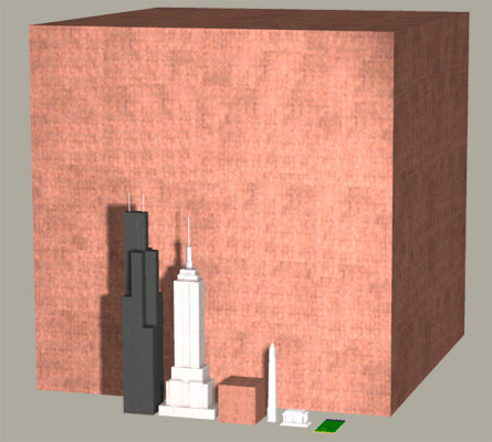
This is a cube of copper pennies 2,730 feet long on each side. The smaller cube (next to the Empire State Building) represents 1 trillion pennies. (See The MegaPenny Project).
Current estimates of brain connectivity often fail to take into account the brain’s mercurial makeup. The brain possesses an extraordinary ability to modify its own structure and function in response to change, both as the result of external events and in accordance with the organism’s innate developmental blueprint.
Mapping networks at the level of connections got its start way back in the 70s with the study of the roundwormC. elegans. More recently the field of connectomics has seen rapid rise in part due to computational advances that allow for the semi-automated collection and analysis of previously unheard of volumes of data. Here I describe some of the challenges that arise when managing and modeling connectome data.
Elegant Worms

Caenorhabditis elegans is a nematode roundworm, generally slender and circular in cross section. It is non-pathogenic and grows to about 1 mm in length. While C. elegans is about as primitive an organism as can be, it shares many essential characteristics relevant to the study of human biology, in particular to human neurobiology.
By far the most complex organ in C. elegans is its nervous system. Of a total of 959 cells, 301 in C. elegans are neuronal. 20 of these are located in the organism’s pharynx (which has its own nervous system). The remaining 281 make up its various head and tail ganglia along with additional ganglia running along its main longitudinal axis.
As a species, C. elegans is remarkably consistent in terms of anatomical structure, especially with regard to the number and placement of its neurons. That is to say, the neurons of any one instance of C. elegans is functionally identical to that of any other. Such consistency has allowed researchers to amass a large and increasingly accurate portrait of C. elegans systems biology over time. Furthermore, all of this information is available to whomever is interested (though you have to look for it).
Constancy of cell number and of cell position from individual to individual is an attribute known as eutely. Eutelic organisms have a fixed number of somatic cells when they reach maturity, the exact number of which is constant for any individual of the species.
Enough talk, let’s have a look at the data.
Data ‘R’ Us
Here I’ll use the R language to help develop some initial insight into the connectome dataset. Before we can use R we first need to get the data into R and luckily it supports all sorts of data formats.
- Flat files can be imported into R with functions like read.table() and read.csv() from the pre-installed utils package. The packages used to import flat file data in R are readr and fread.
- Excel files are imported into R with either the readxl package, gdata or with the XLConnect package.
- The haven package lets you import SAS, STATA and SPSS data files into R.
- We can connect to a database using RMySQL, RpostgreSQL or the ROracle packages. For graph-based database like Neo4J there’s RNeo4j.
- Web scrapers can try out rvest.
The following R script loads a CSV file containing an abridged version of the complete C. elegans dataset.
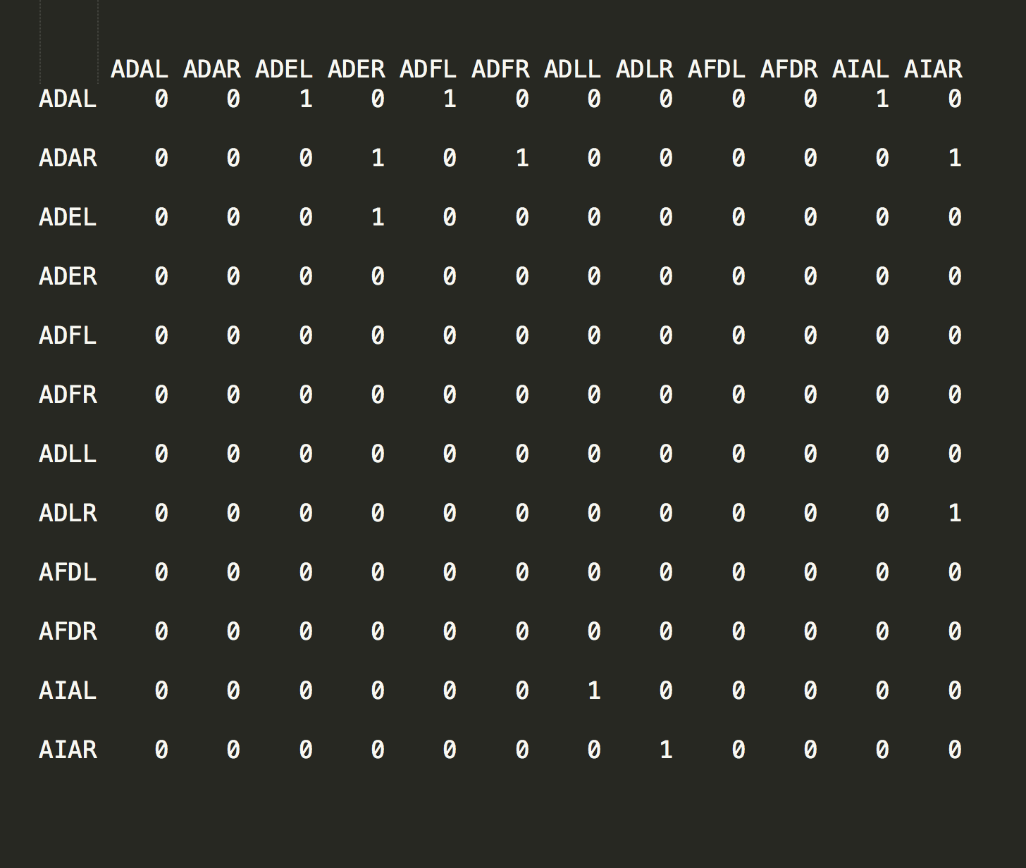
Over time C. elegans’ eutelic property has allowed every cell in the organism to be carefully plotted and catalogued by researchers. This effort has resulted in each cell being labeled with a proper name - ADAL, ADAR, ADEL, etc - and a position in the organism that is consistent from one instance to the next.
After coercing the data into matrix form (line 20) we create an adjacency graph object in line 23. From this we can see that these are indeed connected data.
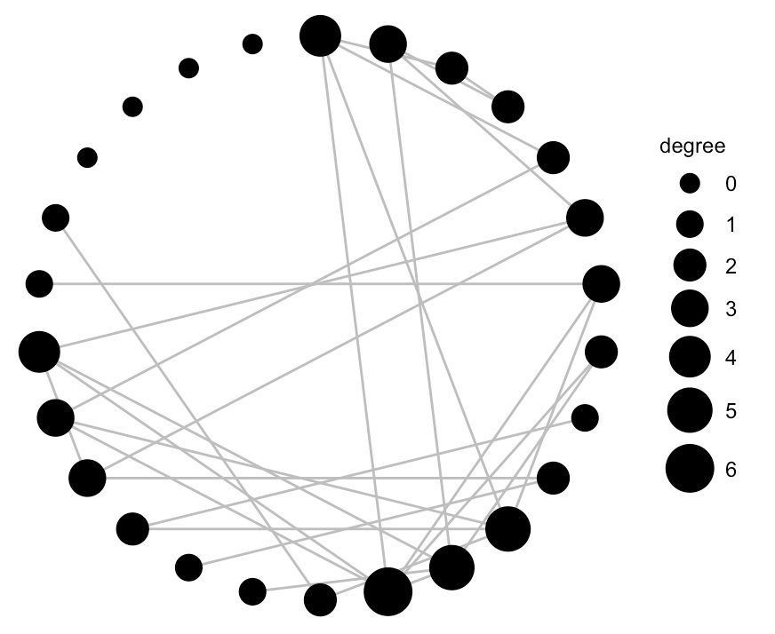
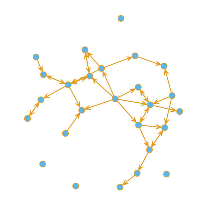
A quick plot reveals that some nodes are more highly connected than others. Bear in mind this is just a sample of the complete dataset.
Finally, we can use ggnet() to hone in a bit on the degree of connectivity. The ggnet and ggnet2 packages allow us to visualize networks as ggplot2 objects.