Predicting Crop Yield From The Sky

06 May 2021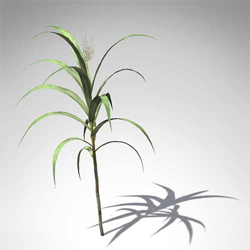

Introduction

I’m sharing a series of posts that document my experience running a two-year agricultural research grant. This project was funded through the Sustainable Agriculture Research and Education SARE section of USDA and considers the application and use of low-cost vegetation indices such as NDVI (more on that later). It was motivated by two important issues in sugarcane farming: 1) seasonal nitrogen input represents a significant cost to farmers; 2) excess nitrogen in the environment alters ecosystems and potentially harms human health. Learning how to manage nitrogen application better is thus motivated by the economics of sugarcane agriculture as well as by the need to address an ongoing environmental issue. For all you agri-geeks out there some of what follows includes reference to the software and code we used to develop and derive our results.

Background

Our crop is sugarcane (Saccharum officinarum). First introduced into the Americas in 1751 it is the highest valued row-crop in the state of Louisiana. While recent years have witnessed a decline in overall sugarcane acreage, crop values have remained stable due to increases in yield. Since increased yield is attributable mainly to the addition of nitrogen fertilizer, how we manage N application is relevant to farmers (in terms of the economics) and to everyone else (in terms of the environment).

Goals

Our study goal was to determine whether low-cost aerial NDVI and other indices could accurately correlate variable N rates when applied to sugarcane. A secondary goal was to determine if such analysis was useful in predicting the yield potential of a future crop. Our work was carried out with the intention of revealing techniques that are affordable, accessible to ordinary farmers and, most importantly, effective.

We asked two questions:

• Can variable nitrogen rates be correlated with multi-spectral imagery?

• Are models of acquired multi-spectral imagery predictive of yield?

To answers these questions a study area was set aside, planted and harvested over two three successive seasons. We used a Latin Square design divided into 30 sections over an area of 1200 by 60 ft. Here is a overview of the area located in Houma, LA.

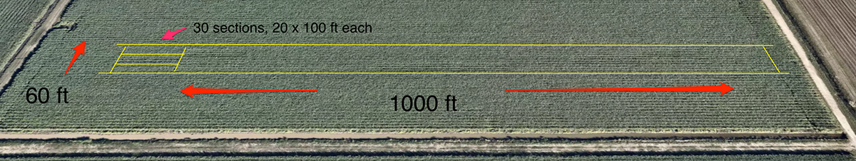
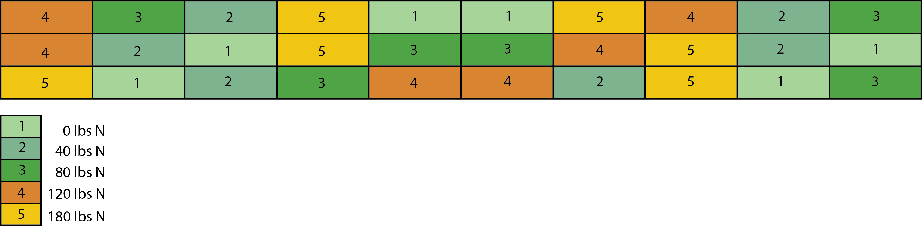
As indicated below five levels of nitrogen fertilization (0, 40, 80, 120 and 180 kg·N·ac−1) were applied in a trial setup with six replicates. This gave us 30 individual plots (100 × 20 sq ft each) making a total trial size of ~1.5 acres.

Tools

Creating a vegetation index first requires getting a camera into the air. As we progressed we used kites, balloons and ultimately an unassisted aerial vehicle (a drone). We created our own multi-spectral cameras along with rigs needed to reproducibly fly them. Ultimately we got help from the folks at Micasense and used their multi-spectral camera, the Sequoia:

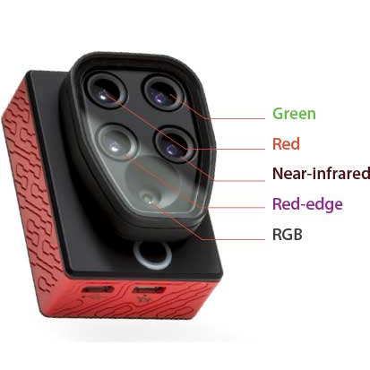
The Sequoia is about the size of a GoPro camera. It’s lightweight enough to fly from a consumer-style drone such as the 3DR Solo. Flying this camera over a field allowed us to collect light reflected in a variety of ways. The Sequoia is sensitive in the Green, Red, Near-infrared and RedEdge bands and by manipulating these bands we created different vegetation indices, one of which is known as the NRG. Most folks are familiar with RGB images but in an NRG image the standard RGB colors (Red-Green-Blue) are exchanged for a different set of color bands: NIR (Near-infrared), Red and Green. Here is an example NRG image:

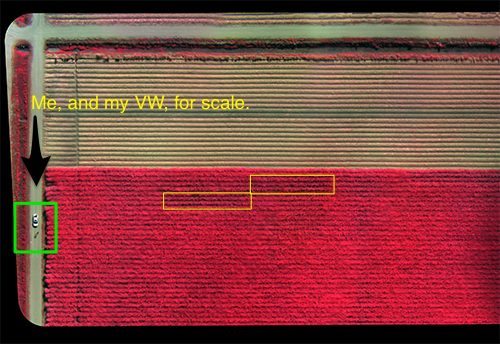
The image above is a composite NRG of a sugarcane field taken on a clear day in late October, 2018. It’s made up of many smaller images in a process involving orthorectification and image-stitching. The two yellow rectangles are the test plots. The green square highlights my white Jetta (and me).

Data

Completing this grant involved many long days in a sugarcane field gathering data but it also required time in front of a computer screen trying to make sense of the data. The following is a code snippet that acts to separate each band of light from the original ‘raw’ data file that’s produced by the Sequoia camera. This is just one part of a much larger image-processing pipeline developed to help automate the work.

The process of separating individual bands of light, stitching together hundreds of smaller images, and running computational methods over the result ultimately produces an image like the one shown below. This image (acquired on July 28th, 2017) shows the full study grid as an NRG image at the height of the growing season.

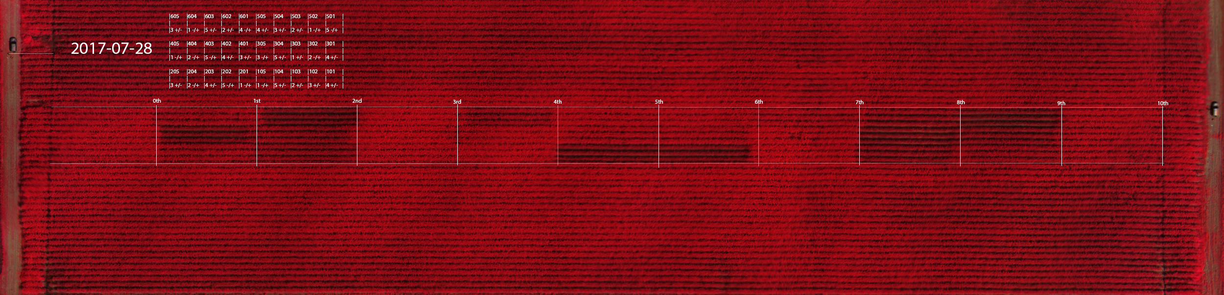
If you look closely you can see a car that appears twice in the image - once in the upper-left and again at the far-right. The study area was too long (1200ft) to be covered in a single flight; it had to be flown twice during each capture - once for the left half and once for the right. We would set up and fly one side, pack everything up and drive to the other and fly again.

A more interesting observation are the shades of red color visible in different parts of the grid. Earlier I mentioned how we treated sections of the area (each about 100 ft by 20 ft) with varying amounts of nitrogen fertilizer. The shades of red signify different intensities of near-infrared light reflected from each section. The treatment of 0 kg·N·ac−1 (#1 in the colored grid at the start of this post) appears as a visible pattern and reveals that differing amounts of nitrogen fertilizer are discernable in terms of the amount of NIR light they reflect. In the next post I’ll explain why.

The Datum

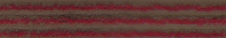
Before moving on I show an image of a single treated section. After going to the trouble of stitching hundreds of images together we had to cut the image up again into smaller samples for statistical analysis. The section above represents a single treatment (one ‘datum’) gathered on a specific day during the sugarcane growing season from late April to mid-November. More than a dozen useable samples per treatment from this field were captured (30 times 12, ~360). Each is spaced in time as evenly as weather permitted, starting a week prior to fertilization and ending four days before the harvest.