
Luigi In Orbit
13 Dec 2018Here I’ll lay the groundwork for a series of posts that will detail how Luigi can be used to orchestrate a more complex set of tasks. In this case a Luigi pipeline helps coordinate the periodic search and retrieval of LANSAT 8 image data. It then prepares that data for upload ontoS3, runs scikit-image and scikit-learn analytics on it, and finally dumps the output so that an API endpoint can serve up the result (through a custom Flask web app). I don’t expect readers to understand how all these separate technologies work. How Luigi glues them together is the point. Primarily, I hope to demonstrate that a tool like Luigi can help shield the data engineer from knowing each and every detail regarding how a pipeline actually functions. Before we open up the hood some background is in order.
Awesome Bands
About a year ago Amazon Web Services began providing up-to-date access to Landsat 8 data via their (highly reliable) AWS infrastructure. The AWS open data initiative includes an extensive archive of Landsat 8 imagery - including individual spectral bands not previously available - allowing anyone access to this valuable information via predictable download endpoints.
Landsat 8 imagery is an incredibly powerful resource. People from around the world have come to rely on it for everything from evaluating drought and predicting agricultural yields to tracking conflict.
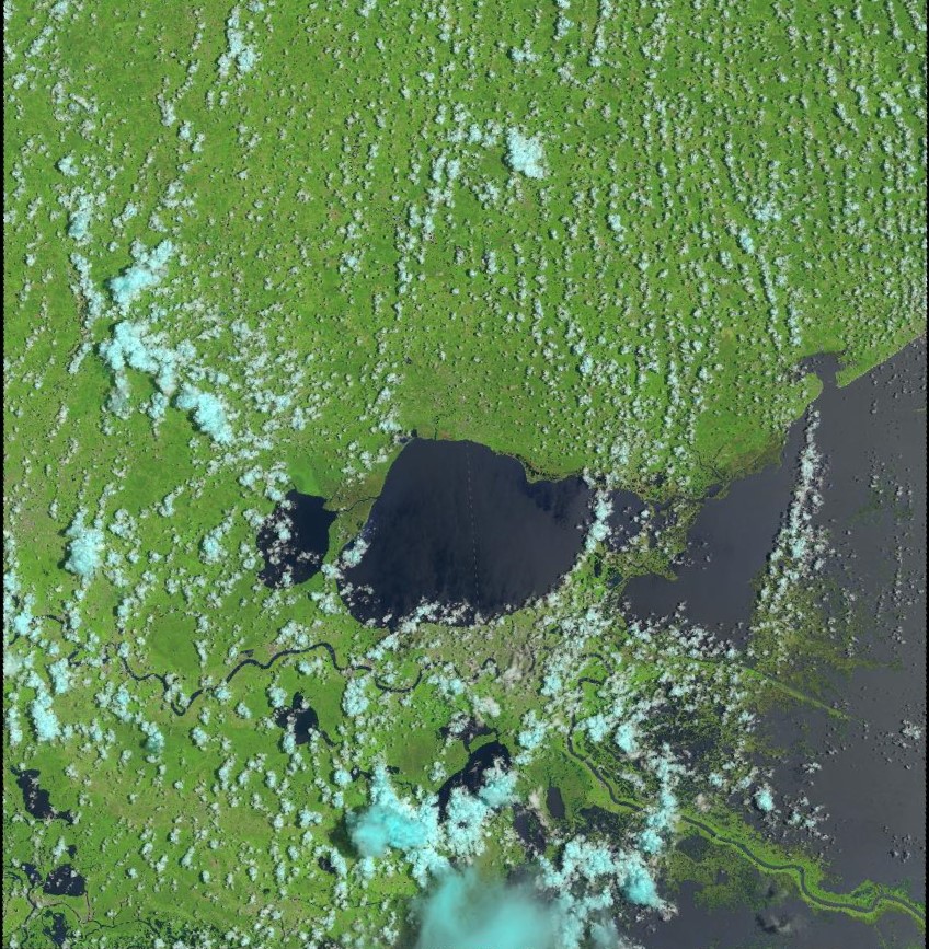
Landsat 8 provides moderate-resolution imagery of Earth’s surface, from 15 metres (panchromatic) to 30 metres (multispectral) to 100 metres (thermal) per pixel. (The above is a capture of southeast Louisiana roughly centered on Lake Ponchartrain). The term per pixel refers to the ground sample distance or GSD which is a way of relating distance between pixel centers to actual distances measured on the ground. For example, in an image with a one-meter GSD, adjacent pixel locations are 1 metre apart on the ground. In the above, each pixel represents a 15 x 15 m “box”, or 2421 square feet (or the size of an average condo in Manhattan).
Landsat 8 operates in the visible, near-infrared, short wave infrared, and thermal infrared spectrums (9 bands total). For the purposes of this project we are interested only in the red, green and near-infrared bands. The following chart specifies several bands with regard to the satellite’s Operational Land Imager (OLI).
| Spectral Band | Wavelength | Resolution | Solar Irradiance |
|---|---|---|---|
| Band 8 - Panchromatic | 0.500 – 0.680 µm | 15 m | 1739 W/(m²µm) |
| Band 2 - Blue | 0.450 – 0.515 µm | 30 m | 1925 W/(m²µm) |
| Band 3 - Green | 0.525 – 0.600 µm | 30 m | 1826 W/(m²µm) |
| Band 4 - Red | 0.630 – 0.680 µm | 30 m | 1574 W/(m²µm) |
| Band 5 - Near Infrared | 0.845 – 0.885 µm | 30 m | 955 W/(m²µm) |
Panchromatic is the combination of all human-visible wavelengths. While containing wavelengths normally associated with familiar RGB photography, an image from the pan band is more similar to black-and-white film in the way it combines light from the visible spectrum into a single measure of overall reflectance. The SI unit of irradiance is the watt per square metre (W/m2).
Getting Started
Landsat data can be a challenge to work with, especially for individuals or small organizations lacking tools. It can take a novice a day (or a week) to collect, composite, color correct, and sharpen Landsat 8 imagery. To help I’m using an open source toolkit called landsat-util. While this is not the only way to gain access to Landsat (more on that later) this particular tool makes it very easy to search, download, and process directly from the command line.
Searching with landsat-util makes us of the landsat-api which enables making geospatial, date and text queries on Landsat-8 metadata. (The metadata is released in csv format by USGS on a daily basis.)
Here is an example of searching with landsat-util:
>> landsat search
  --start 07/03/2016
  --end 07/10/2016
  --lat 29.909273
  --lon -90.920771
The output of above is a JSON response which can be stored as out.json on the local file system. Next we parse the file and pull out those elements that are of interest.
The result is a list of (date, sceneID) tuples filtered such that only dates where less than 20% cloud cover occurred are captured. This filtering step is important for later in the processing chain.
We’ve searched Landsat for imagery taken between July 3 and July 10, roughly centered on New Orleans, and filtered the result for cloud cover. The next step is to download the filtered images and process them. Landsat 8 imagery acquired before 2015 is downloaded from Google Earth Engine while anything afterwards comes from AWS Public Data Sets. Here I am asking for a specific sceneID (returned as the result of the previous search) and requesting bands 3, 4 and 5.
>> landsat download
  LC80220402016185LGN00
  --bands 345
I’ve said nothing about the supporting software required to run landsat-util. The tool requires some amount of infrastructure and there may be performance and dependency issues when running locally. For now I’ll issue a promissary note with the suggestion that to more easily get landsat-util up and running, Docker is your friend.